2 A Pragmatic Guide for Analysis with crawl
The crawl package is designed and built with the idea that it should be
accessible and useful to a research biologist with some intermediate R
skills and an understanding of the basic statistical theory behind
the analysis of animal movement. This portion of the book will focus on
providing the user with suggested principles, workflows, and pragmatic
approaches that, if followed, should make analysis with crawl more
efficient and reliable.
Telemetry data are collected on a wide range of species and come in a number of formats and data structures. The code and examples provided here were developed from data the authors are most familiar with. You will very likely NOT be able to just copy and paste the code and apply to your data. We suggest you focus more on understanding what the code is doing and then write your own version of the code to meet your data and your research needs.
This content is broken up in the following sections:
- Analysis and Coding Principles
- Assembling Source Data
- Tidy Data for Telemetry
- Preparing Input Data for
crawl - Determining Your Model Parameters
- Exploring and Troubleshooting Model Results
- Predicting a Movement Track
- Simulating Tracks from the Posterior
- Visualization of Results
2.1 Analysis and Coding Principles
As with anything in science and R, there are a number of right ways to
approach a problem. The workflows and principles outlined here aren’t the only
way to use crawl. However, this content has been developed after years of
working with researchers and troubleshooting common issues. For most users,
following this guide will prove a successful endeavor. More advanced users
or those with specific needs should feel free to refer to this as a starting
point but then expand to meet their need.
2.1.1 Source Data are Read Only
Source data should not be edited. In many cases, the financial and personal investment required to obtain these data is significant. In addition, the unique timing, location, and nature of the data cannot be replicated so every effort should be employed to preserve the integrity of source data as they were collected. All efforts should be made to also insure that source data are stored in plain text or well described open formats. This approach provides researchers confidence that data will be available and usable well into the future.
2.1.2 Script Everything
In all likelihood, the format of any source data will not be condusive to
established analytical procedures. For example, crawl cannot accept a raw
data file downloaded from ArgosWeb or the Wildlife Computers Data Portal. Some
amount of data carpentry is required. Keeping with the principles of
reproducibility, all data assembly and carpentry should be scripted. Here, we
rely on the R programming language for our scripts, but Python or other
similar languages will also meet this need.
2.1.3 Document Along the Way
Scripting the data assembly should be combined with an effort to properly
document the process. Documentation is an important component of reproducibility
and, if done as part of the scritping and development process, provides an
easier workflow for publishing results and data to journals and repositories.
The rmarkdown, bookdown, and knitr packages provide an excellent
framework for combining your R scripts with documentation. This entire
book is written with bookdown and knitr.
2.1.4 Embrace the Tidyverse
The tidyverse describes a set of R packages developed by, or in association with, Hadley Wickham. Tidy data principles are outlined in a 2014 paper published in the Journal of Statistical Software. The key tennants of tidy data are:
- Each variable forms a column.
- Each observation forms a row.
- Each type of observational unit forms a table.
Location data from telemetry deployments often follows this type of structure: each location estimate is a row and the columns all represent variable attributes associated with that location. Additionally, the location data are usually organized into a single table. Behavior data, however, often comes in a less structured format. Different behavior type data are sometimes mixed within a single table and column headings do not consistently describe the same variable (e.g. Bin1, Bin2, etc). There are valid reasons for tag vendors and data providers to transmit the source data in this way, but the structure is not condusive to analysis.
The tidyverse package is a wrapper for a number of separate packages that each
contribute to the tidy’ing of data. The tidyr, dplyr, readr, and purrr
packages are key components. In addition, the lubridate package (not included
in the tidyverse package) is especially useful for consistent maninpulation
of date-time values. More information and documentation for the packages can be
found at the tidyverse.org website.
2.1.5 Anticipate Errors & Trap Them
Use R’s error trapping functions (try() and tryCatch()) in areas of your
code where you anticipate parsing errors or potential issues with convergence
or fit. The purrr::safely() function also provides a great service.
2.2 Assembling Source Data
Where and how you access the source data for your telemetry study will depend on the type of tag and vendor. Argos location data is available to users from the Argos website and many third party sites and respositories (e.g. movebank, sea-turtle.org) have API connections to ArgosWeb that can faciliate data access. Each tag manufacturer often has additional data streams included within the Argos transmission that require specific software or processing to translate. Both the Sea Mammal Research Unit (SMRU) and Wildlife Computers provide online data portals that provide users access to the location and additional sensor data.
Regardless of how the data are retrieved, these files should be treated as read only and not edited. ArgosWeb and vendors have, typically, kept the data formats and structure consistent over time. This affords end users the ability to develop custom processing scripts without much fear the formats will change and break their scripts.
2.2.1 Read In CSV Source Data
Here we will demonstrate the development of such a script using data downloaded
from the Wildlife Computers (Redmond, Washington, USA) data portal. All data are
grouped by deployment and presented in various comma-separated files. The
*-Locations.csv contains all of the Argos location estimates determined for
the deployment. At a minimum, this file includes identifying columns such as
DeployID, PTT, Date, Quality, Type, Latitude, and Longitude. If
the Argos Kalman filtering approach has been enabled (which it should be for any
modern tag deployment), then additional data will be found in columns that
describe the error ellipses (e.g. Error Semi-major axis, Error Semi-minor axis, Error Ellipse orientation). Note, if the tag transmitted GPS/FastLoc
data, this file will list those records as Type = 'FastGPS'.
The other file of interest we will be working with is an example *-Histos.csv.
These files include dive and haul-out behavior data derived from sensors on the
tag. Most notably, the pressure transducer (for depth) and the salt-water switch
(for determining wet/dry status). We will focus on processing this file to
demonstrate how we can properly tidy our data.
We will rely on the tidyverse set of packages plus purrr and lubridate
to make reading and processing these files easier and more reliable. Since we are
working with spatial data, the sf package will be used (as well as a few
legacy functions from the sp package).
if(!require(devtools)) install.packages('devtools')
library(tidyverse)
library(lubridate)
library(sp)
library(sf)
The readr includes the read_csv() function which we will rely on to read
the csv data into R.
2.2.2 Specify Column Data Types
The readr::read_csv() function tries to interpret the proper data types for
each of the columns and provides us the column specifications it determined. In
most cases, the function gets this correct. However, if we examine the cols()
specification selected, we see that the Date column was
read in as a character data type.
To correct this, we need to provide our own cols() specification. We can do
this by simply modifying the specification readr::read_csv() provided us. In
this case, we want the Date column to rely on col_datetime and to parse
the character string using the format %H:%M:%S %d-%b-%Y.
my_cols <- cols(
  DeployID = col_character(),
  Ptt = col_integer(),
  Instr = col_character(),
  Date = col_datetime("%H:%M:%S %d-%b-%Y"),
  Type = col_character(),
  Quality = col_character(),
  Latitude = col_double(),
  Longitude = col_double(),
  `Error radius` = col_integer(),
  `Error Semi-major axis` = col_integer(),
  `Error Semi-minor axis` = col_integer(),
  `Error Ellipse orientation` = col_integer(),
  Offset = col_character(),
  `Offset orientation` = col_character(),
  `GPE MSD` = col_character(),
  `GPE U` = col_character(),
  Count = col_character(),
  Comment = col_character()
)

tbl_locs <- readr::read_csv(path_to_file,col_types = my_cols)
2.2.3 Import From Many Files
In most instances you’ll likely want to read in data from multiple deployments.
The purrr::map() function can be combined with readr::read_csv() and
dplyr::bind_rows() make this easy.
tbl_locs <- dir('examples/data/', "*-Locations.csv", full.names = TRUE) %>%
  purrr::map(read_csv,col_types = my_cols) %>%
  dplyr::bind_rows()

tbl_locs %>% dplyr::group_by(DeployID) %>%
  dplyr::summarise(num_locs = n(),
            start_date = min(Date),
            end_date = max(Date))
## # A tibble: 2 x 4
## DeployID num_locs start_date end_date
## <chr> <int> <dttm> <dttm>
## 1 PV2016_3019_16A0222 3064 2016-09-21 02:54:02 2017-02-15 08:15:22
## 2 PV2016_3024_15A0909 976 2016-09-22 02:48:00 2017-02-15 05:06:202.3 Tidy Data for Telemetry
A key tennat of tidy data is that each row represents a single observation. For
location data, regardless of the data source, this is typical of the source data
structure. Each line in a file usually represents a single location estimate at
a specific time. So, there’s very little we need to do in order to get our
tbl_locs into an acceptable structure.
2.3.1 Standard Column Names
One thing we can do, is to adjust the column names so there are no spaces or
hyphens. We can also drop everything to lower-case to avoid typos. To do this
we will create our own function, make_names(), which expands on the base
function make.names(). We also want to change the date column to a more appropriate and less confusing date_time.
## This function is also available within the crawlr package
make_names <- function(x) {
  new_names <- make.names(colnames(x))
  new_names <- gsub("\\.", "_", new_names)
  new_names <- tolower(new_names)
  colnames(x) <- new_names
  x
}

tbl_locs <- dir('examples/data/', "*-Locations.csv", full.names = TRUE) %>%
  purrr::map(read_csv,col_types = my_cols) %>%
  dplyr::bind_rows() %>%
  make_names() %>%
  dplyr::rename(date_time = date) %>%
  dplyr::arrange(deployid, date_time)
At this point, our tbl_locs is pretty tidy and, other than a few final steps,
ready for input into the crawl::crwMLE() function. The *-Histos.csv file,
however, has a messy, horizontal structure and will require some tidying. The
tidyr package has a number of options that will help us. But, first let’s look
closer at the structure of a typical *-Histos.csv.
2.3.2 Tidy a Messy ‘Histos’ File
Wildlife Computers provides a variety of data types within this file structure.
Because the details of each data type are subject to tag programming details, the
data structure places observations into a series of Bin1, Bin2, ..., Bin72
columns. What each Bin# column represents depends on the data type and how the
tags were programmed. For instance, a Dive Depth record represents the number
of dives with a maximum depth within the programmed depth bin range.
Time At Depth (TAD) represents the number of seconds spent within a particular
programmed depth bin range. Each record represents a period of time that is also
user programmable.
While this messy data structure is an efficient way of delivering the data to
users, it violates the principles of tidy data strucutes and presents a number
of data management and analysis challenges. We are going to focus on a process
for tidying the Percent or 1Percent timeline data as this information can
be incorporated into the crawl::crwMLE() model fit. The same approach should
be adopted for other histogram record types and the wcUtils
package provides a series of helper
functions developed specifically for this challenge.
The Percent/1Percent timeline data are presented within the *-Histos.csv
file structure as 24-hour observations — each record represents a 24-hour UTC
time period. Within the record, each Bin# represents an hour of the day from
00 through 23. The values recorded for each Bin# column represent the
percentage of that hour the tag was dry (out of the water). This data structure
violates the tidy principles of requiring each record represent a single
observation and that each column represent a single variable.
Let’s start by reading the data in to R with readr::read_csv() as before.
Note, we again rely on a custom cols() specification to insure data types
are properly set. And, since we are only interested in Bin columns 1:24, we
will select out the remaining columns.
my_cols <- readr::cols(
  DeployID = readr::col_character(),
  Ptt = readr::col_character(),
  DepthSensor = readr::col_character(),
  Source = readr::col_character(),
  Instr = readr::col_character(),
  HistType = readr::col_character(),
  Date = readr::col_datetime("%H:%M:%S %d-%b-%Y"),
  `Time Offset` = readr::col_double(),
  Count = readr::col_integer(),
  BadTherm = readr::col_integer(),
  LocationQuality = readr::col_character(),
  Latitude = readr::col_double(),
  Longitude = readr::col_double(),
  NumBins = readr::col_integer(),
  Sum = readr::col_integer(),
  Bin1 = readr::col_double(), Bin2 = readr::col_double(), Bin3 = readr::col_double(),
  Bin4 = readr::col_double(), Bin5 = readr::col_double(), Bin6 = readr::col_double(),
  Bin7 = readr::col_double(), Bin8 = readr::col_double(), Bin9 = readr::col_double(),
  Bin10 = readr::col_double(), Bin11 = readr::col_double(), Bin12 = readr::col_double(),
  Bin13 = readr::col_double(), Bin14 = readr::col_double(), Bin15 = readr::col_double(),
  Bin16 = readr::col_double(), Bin17 = readr::col_double(), Bin18 = readr::col_double(),
  Bin19 = readr::col_double(), Bin20 = readr::col_double(), Bin21 = readr::col_double(),
  Bin22 = readr::col_double(), Bin23 = readr::col_double(), Bin24 = readr::col_double(),
  Bin25 = readr::col_double(), Bin26 = readr::col_double(), Bin27 = readr::col_double(),
  Bin28 = readr::col_double(), Bin29 = readr::col_double(), Bin30 = readr::col_double(),
  Bin31 = readr::col_double(), Bin32 = readr::col_double(), Bin33 = readr::col_double(),
  Bin34 = readr::col_double(), Bin35 = readr::col_double(), Bin36 = readr::col_double(),
  Bin37 = readr::col_double(), Bin38 = readr::col_double(), Bin39 = readr::col_double(),
  Bin40 = readr::col_double(), Bin41 = readr::col_double(), Bin42 = readr::col_double(),
  Bin43 = readr::col_double(), Bin44 = readr::col_double(), Bin45 = readr::col_double(),
  Bin46 = readr::col_double(), Bin47 = readr::col_double(), Bin48 = readr::col_double(),
  Bin49 = readr::col_double(), Bin50 = readr::col_double(), Bin51 = readr::col_double(),
  Bin52 = readr::col_double(), Bin53 = readr::col_double(), Bin54 = readr::col_double(),
  Bin55 = readr::col_double(), Bin56 = readr::col_double(), Bin57 = readr::col_double(),
  Bin58 = readr::col_double(), Bin59 = readr::col_double(), Bin60 = readr::col_double(),
  Bin61 = readr::col_double(), Bin62 = readr::col_double(), Bin63 = readr::col_double(),
  Bin64 = readr::col_double(), Bin65 = readr::col_double(), Bin66 = readr::col_double(),
  Bin67 = readr::col_double(), Bin68 = readr::col_double(), Bin69 = readr::col_double(),
  Bin70 = readr::col_double(), Bin71 = readr::col_double(), Bin72 = readr::col_double()
)

tbl_percent <- dir('examples/data/',
    "*-Histos.csv",
    full.names = TRUE) %>%
  purrr::map(read_csv,col_types = my_cols) %>%
  dplyr::bind_rows() %>%
  make_names() %>%
  dplyr::select(-(bin25:bin72)) %>%
  dplyr::arrange(deployid, date)
2.3.3 Gathering Data with tidyr
Now that our percent timeline data are in R, we can work to tidy the data
structure using the tidyr::gather() function. This function requires that we
provide character names for the key and value columns to create. We then
specify which columns will be gathered into those key-value paired columns.
In this case, our new columns will be bin and percent_dry and we will
gather the values from all of the columns that start with the character string
bin.
Since we know that each bin column represents an hour of the day, we can also
improve our data structure by changing the value of date_hour (note we rename
date to date_hour) to reflect this. We accomplish this by creating a simple
lookup table (tibble) that relates each bin column to the hour of day it
represents. The dplyr::left_join() function is used to match and merge this
with our tbl_percent and then we add the hour value to each date_hour
value with the dplyr::mutate() and lubridate::hours() functions.
## Create a tbl_df that Relates Bin Columns to Day Hours
bins <- tibble(bin = paste("bin",1:24,sep = ""),hour = 0:23)

## Chain Together Multiple Commands to Create Our Tidy Dataset
tbl_percent <- tbl_percent %>%
  tidyr::gather(bin,percent_dry, starts_with('bin')) %>%
  dplyr::left_join(bins, by = "bin") %>%
  dplyr::rename(date_hour = date) %>%
  dplyr::mutate(date_hour = date_hour + lubridate::hours(hour)) %>%
  dplyr::select(deployid,date_hour,percent_dry) %>%
  dplyr::group_by(deployid, date_hour) %>%
  dplyr::summarize(percent_dry = mean(percent_dry)) %>%
  dplyr::ungroup() %>%
  dplyr::arrange(deployid,date_hour)
Examining tbl_percent, we see that the layout is now more vertical and more
in line with tidy principles
## # A tibble: 5,564 x 3
##    deployid            date_hour           percent_dry
##    <chr>               <dttm>                    <dbl>
##  1 PV2016_3019_16A0222 2016-09-21 02:00:00          NA
##  2 PV2016_3019_16A0222 2016-09-21 03:00:00          NA
##  3 PV2016_3019_16A0222 2016-09-21 04:00:00         100
##  4 PV2016_3019_16A0222 2016-09-21 05:00:00         100
##  5 PV2016_3019_16A0222 2016-09-21 06:00:00         100
##  6 PV2016_3019_16A0222 2016-09-21 07:00:00          30
##  7 PV2016_3019_16A0222 2016-09-21 08:00:00          20
##  8 PV2016_3019_16A0222 2016-09-21 09:00:00          10
##  9 PV2016_3019_16A0222 2016-09-21 10:00:00          10
## 10 PV2016_3019_16A0222 2016-09-21 11:00:00          10
## # ... with 5,554 more rows
2.3.4 Visualizing Source Data
To further explore our imported data and confirm there aren’t any remaining
issues to address, we can create visual representations of the data. The first
plot will rely on the spatial features within ggplot2 and an extension to the
package, ggspatial to create a plot of the tbl_locs object. The second plot
will create a heatmap of tbl_percent values.
The sf package provides the bulk of our spatial data framework. This is not
intended to be a full sf tutorial, but, where possible we will highlight a
few features and functions to explain the workflow. Users are encouraged to
spend significant time exploring and understanding the sf package through
existing documentation and several examples and blog posts available online.
Here, we are simply creating an sf_locs object via the sf::st_as_sf()
function. We specify the coordinate columns and then indicate the projection
of the data is geographic (lat/lon) as indicated by the 4326 epsg code.
In addition to points, it is often useful to organize the point data into
separate tracks for each deployment. The code to derive tracks from point data
within sf is a bit more complicated but is demonstrated below. The sf_lines
object is, essentially, a data frame with each row representing a single line
from a single deployment.
sf_locs <- sf::st_as_sf(tbl_locs, coords = c("longitude","latitude")) %>%
  sf::st_set_crs(4326)

sf_lines <- sf_locs %>%
  dplyr::arrange(deployid, date_time) %>%
  sf::st_geometry() %>%
  sf::st_cast("MULTIPOINT",ids = as.integer(as.factor(sf_locs$deployid))) %>%
  sf::st_cast("MULTILINESTRING") %>%
  sf::st_sf(deployid = as.factor(unique(sf_locs$deployid)))
(ref:map-locs-fig-cap) An interactive map of observed satellite telemetry locations from two harbor seals in the Aleutian Islands.
esri_ocean <- paste0('https://services.arcgisonline.com/arcgis/rest/services/',
                     'Ocean/World_Ocean_Base/MapServer/tile/${z}/${y}/${x}.jpeg')

ggplot() +
  annotation_map_tile(type = esri_ocean,zoomin = 1,progress = "none") +
  layer_spatial(sf_lines, size = 0.75,aes(color = deployid)) +
  scale_x_continuous(expand = expand_scale(mult = c(.6, .6))) +
  scale_color_brewer(palette = "Dark2") +
  theme(legend.position = "none") +
  ggtitle("Observed Argos Location Paths",
          subtitle = "harbor seals (n=2), Aleutian Islands, Alaska, USA")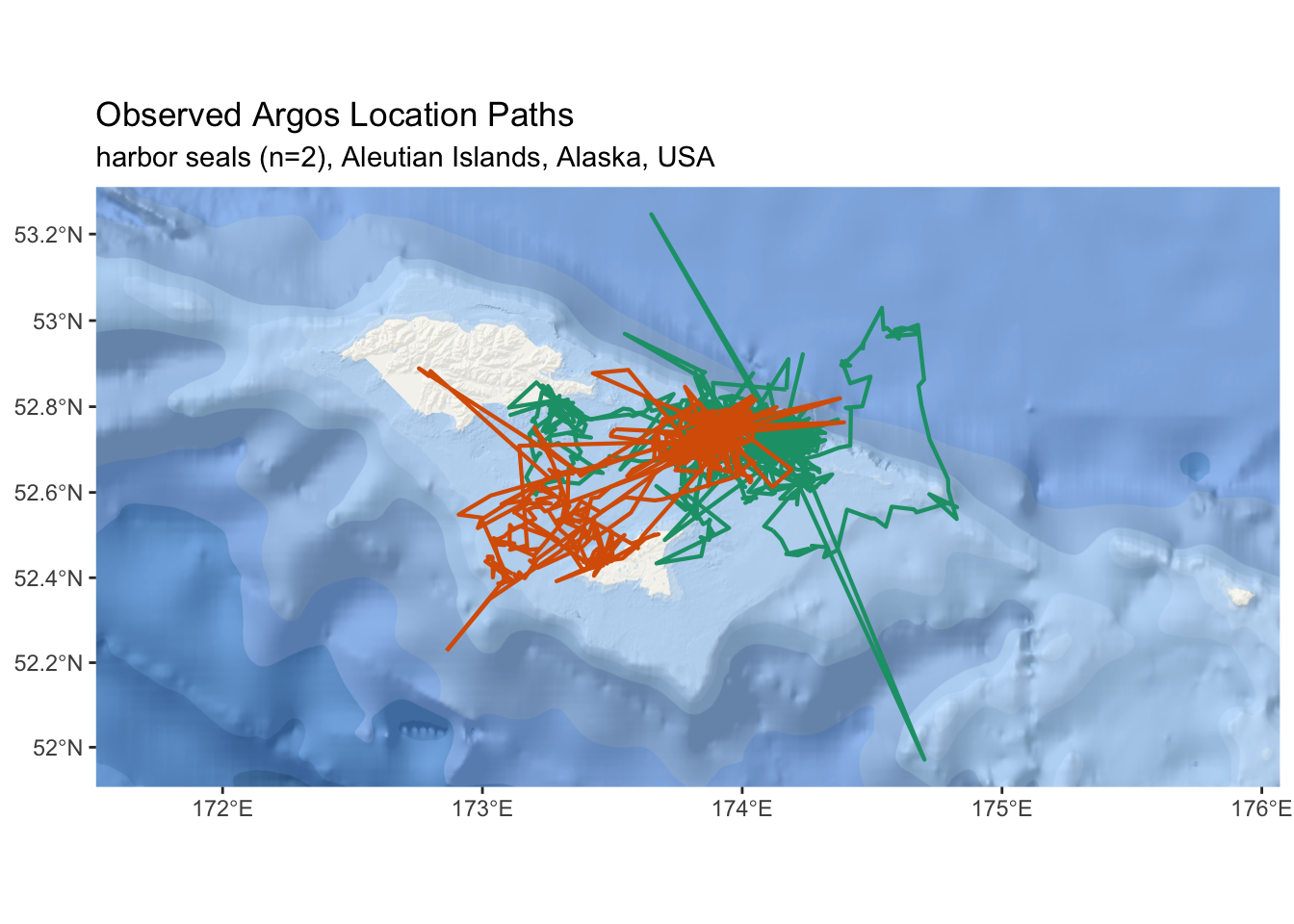
Figure 2.1: (ref:map-locs-fig-cap)
(ref:percent-timeline-heatmap) Depiction of hourly percent dry observations for two satellite tags deployed on harbor seals in the Aleutian Islands.
library(viridis)
p <- tbl_percent %>%
  dplyr::mutate(solar_hour = date_hour + lubridate::dhours(11.5),
                solar_hour = lubridate::hour(solar_hour)) %>%
  ggplot(aes(x = lubridate::date(date_hour),
                           y = solar_hour,
                           fill = percent_dry)) +
  geom_tile() +
  scale_y_continuous(breaks = c(6,12,18)) +
  scale_fill_viridis(name = "Percent Dry",
                     guide = guide_colorbar(
                       title.position = "bottom",
                       barwidth = 25, barheight = 1 )) +
  facet_wrap( ~ deployid, nrow = 2) +
  theme(axis.title = element_text()) +
  ylab("local solar hour") + xlab("") +
  ggtitle(paste("Haul-out Behavior by Local Solar Hour")) +
  theme(panel.grid.major.x = element_blank(),
        legend.position="bottom")
p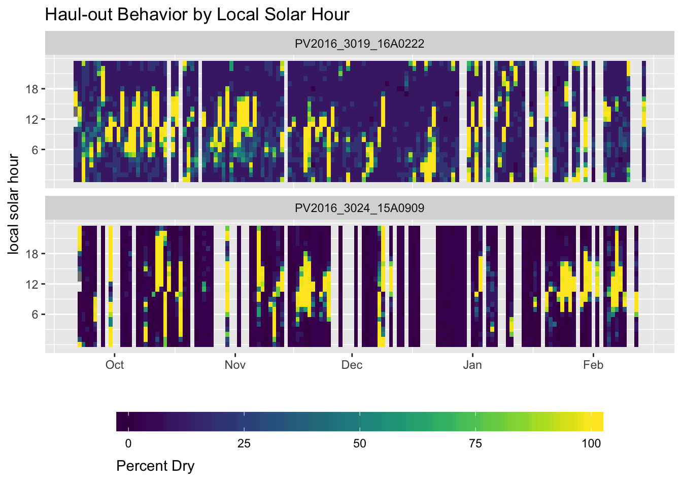
Figure 2.2: (ref:percent-timeline-heatmap)
2.4 Preparing Input Data for crawl
At this point, the tbl_locs object represents the minimal source data
required to fit crawl::crwMLE(). In addition to including location estimates
in the model fit, one can also include an activity parameter. For harbor seals,
we can rely on the percent-timeline data as an indicator of activity — when
the tags are dry for most of an hour, the seal is likely hauled out and not
moving. The crawl::crwMLE() will interpret this as an indication that the
auto-correlation parameter should go to zero.
In this section, we will prepare two input objects for crawl::crwMLE(). The
first will be a spatial object (sf_locs) of location estimates that can be passed
directly. The second, will be a data.frame (tbl_locs_activity) that represents a merge between the location estimates and percent-timeline data.
2.4.1 Error Parameters for GPS Data
Many tags deployed on marine animals now include the option to collect GPS
quality location esimates in addition to Argos. crawl::crwMLE() relies on the
ellipse error parameters provide by Argos, so we need to fill in the GPS
locations with appropriate values. GPS locations from these tags are generally
expected to have an error radius of ~50m as long as the number of satellites
used for the estimate is greater than 4. Below, we will use the dplyr::mutate()
function to fill in these values. While we are at it, we will also remove any
Argos records that do not have associated error ellipse values.
tbl_locs <- tbl_locs %>%
  dplyr::filter(!(is.na(error_radius) & type == 'Argos')) %>%
  dplyr::mutate(
    error_semi_major_axis = ifelse(type == 'FastGPS', 50,
                                   error_semi_major_axis),
    error_semi_minor_axis = ifelse(type == 'FastGPS', 50,
                                   error_semi_minor_axis),
    error_ellipse_orientation = ifelse(type == 'FastGPS', 0,
                                       error_ellipse_orientation)
    )
2.4.2 Known Locations
In many cases, researchers are also knowledgable of the time and location
coordinates of animal release. The Wildlife Computers Data Portal allows this
to be entered and is included as a User record. The error radius one might
specify for this record is dependent on the release situation. In general,
it is best to over estimate this error radius. This record should be the first
location record in the dataset passed to crawl::crwMLE().
Some researchers may also have additional date-times during the deployment
when the location is known (e.g. fur seals returning to a rookery between trips).
In these cases, tbl_locs can be augmented with additional User locations, but
the code example below will need to be customized for each situation. This code
example presumes there is just one User location and that corresponds to the
release/deployment start.
tbl_locs <- tbl_locs %>%
  dplyr::mutate(
    error_semi_major_axis = ifelse(type == 'User', 500,
                                   error_semi_major_axis),
    error_semi_minor_axis = ifelse(type == 'User', 500,
                                   error_semi_minor_axis),
    error_ellipse_orientation = ifelse(type == 'User', 0,
                                       error_ellipse_orientation)
    )

user_dt <- tbl_locs %>% dplyr::rename(release_dt = date_time) %>%
  dplyr::filter(type == 'User') %>% dplyr::select(deployid,release_dt)

tbl_locs <- tbl_locs %>% dplyr::left_join(user_dt, by = 'deployid') %>%
  dplyr::filter(date_time >= release_dt) %>% dplyr::select(-release_dt)

tbl_locs %>% dplyr::group_by(deployid) %>% dplyr::select(deployid,date_time,type) %>%
  dplyr::do(head(.,1))
## # A tibble: 2 x 3
## # Groups: deployid [2]
## deployid date_time type
## <chr> <dttm> <chr>
## 1 PV2016_3019_16A0222 2016-09-21 05:08:00 User
## 2 PV2016_3024_15A0909 2016-09-22 02:48:00 User2.4.3 Duplicate Times
Argos data often contain near duplicate records. These are identified by location
estimates with the same date-time but differing coordinate or error values. In
theory, crawl::crwMLE() can handle these situations, but we have found it is
more reliable to fix these records. The first option for fixing the records
would be to eliminate one of the duplicate records. However, it is often not
possible to reliably identify which record is more appropriate to discard. For
this reason, we advocate adjusting the date-time value for one of the records and
increasing the value by 10 second. To facilitate this, we will rely on the
xts::make.time.unique() function.
make_unique <- function(x) {
  xts::make.time.unique(x$date_time,eps = 10)
}

library(xts)

tbl_locs <- tbl_locs %>%
  dplyr::arrange(deployid,date_time) %>%
  dplyr::group_by(deployid) %>% tidyr::nest() %>%
  dplyr::mutate(unique_time = purrr::map(data, make_unique)) %>%
  tidyr::unnest() %>%
  dplyr::select(-date_time) %>% rename(date_time = unique_time)
2.4.4 Course Speed Filter
This step is optional, but it is very common for Argos data to include obviously
wrong locations (locations that are hundreds of kilometers away from the study area).
Including such obviously wrong locations in the analysis can result in unexpected
issues or problems fitting. For this reason, we recommend a course speed filter
to remove these obviously wrong locations. A typical speed filter might use a
value of 2.5 m/s as a biologically reasonable value for pinnipeds. For this
application, we will use 7.5 m/s and rely on the argosfilter package.
The example code below follows a typical split-apply-combine approach using
functions from the dplyr, tidyr, and purrr packages. This analysis can
be run in series, however, the process lends itself nicely to parallel processing.
The parallel package (included with the distribution of R) would be one option
for taking advantage of multiple processors. However, we want to maintain the
purrr and nested column tibble data structure. The multidplyr package is
in development and available for install via the devtools package and source
code hosted on GitHub.
This is not intended to be a multidplyr tutorial, so some details are left
out. That said, many processes in analysis of animal movement are setup nicely
for parallel processing. We encourage anyone who is doing movement analysis on
datasets with a large number of animals to spend some time learning about the
various parallel processing options within R.
library(purrr)
library(furrr)

future::plan(multiprocess)

tbl_locs <- tbl_locs %>%
  dplyr::arrange(deployid, date_time) %>%
  dplyr::group_by(deployid) %>%
  tidyr::nest()

tbl_locs %>% dplyr::summarise(n = n())
## # A tibble: 1 x 1
## n
## <int>
## 1 2tbl_locs <- tbl_locs %>%
dplyr::mutate(filtered = furrr::future_map(data, ~ argosfilter::sdafilter(
lat = .x$latitude,
lon = .x$longitude,
dtime = .x$date_time,
lc = .x$quality,
vmax = 7.5
))) %>%
tidyr::unnest() %>%
dplyr::filter(filtered %in% c("not", "end_location")) %>%
dplyr::select(-filtered) %>%
dplyr::arrange(deployid,date_time)
tbl_locs %>% dplyr::summarise(n = n())## # A tibble: 1 x 1
## n
## <int>
## 1 37872.4.5 Create a Spatial Object
There are now two package frameworks within R for describing spatial data: sp
and sf. The sp package has been the defacto standard for spatial data in R
and has widespread support in a number of additional packages. The sf package
is new and still in active development. However, the sf package is based on
the more open simple features standard for spatial data. For this reason, and
others, many in the R community feel sf is the future of spatial data in R.
In the previous section, our leaflet map relied on input of an sf object.
The crawl::crwMLE() can accept either a SpatialPointsDataFrame from the
sp package or an sf data.frame of POINT geometry types. Here, we will
focus on the sf package.
Earlier versions of crawl allowed users to pass geographic coordinates (
e.g. latitude, longitude). However, relying on geographic coordinates presents some
problems (e.g. crossing 180 or 0) and requires some assumptions to convert
decimal degrees into meters — the units for the provided error ellipses.
Because of these issues, all data should be provided to the crawl::crwMLE()
as projected coordinates in meter units. Which projection users choose is
dependent upon their study area. For these data, we will go with the North Pole
LAEA Bering Sea projection. This projection is often abbreciated by the epsg
code of 3571. If you don’t know the epsg code for the preferred projection in
your study area, a the spatial reference
website provides a comprehensive catalog of projections and epsg codes.
The sf::transform() function provides an easy method for transforming our
coordinates. After, we can examine the geometry and confirm our coordinate
units are in meters.
## Geometry set for 3787 features
## geometry type:  POINT
## dimension:      XY
## bbox:           xmin: -510531.2 ymin: -4094081 xmax: -369854 ymax: -4034591
## epsg (SRID):    3571
## proj4string:    +proj=laea +lat_0=90 +lon_0=180 +x_0=0 +y_0=0 +datum=WGS84 +units=m +no_defs
## First 5 geometries:
At this point, sf_locs is a valid format for input to crawl::crwMLE().
However, if you want to include the percent-timeline data as an activity
parameter, there’s bit more work to do.
2.4.6 Merging with Activity Data
Since our activity data represent hourly records, we need to create a
date_hour field within tbl_locs as the basis for our join. While we are at
it, we’ll translate the simple feature geometry
for our point coordinates into an x and y column (note the use of a local
function sfc_as_cols() to facilitate this). This addition of an x and y
column is mostly a convenience function that may not be needed in future versions.
sfc_as_cols <- function(x, names = c("x","y")) {
  stopifnot(inherits(x,"sf") && inherits(sf::st_geometry(x),"sfc_POINT"))
  ret <- sf::st_coordinates(x)
  ret <- tibble::as_tibble(ret)
  stopifnot(length(names) == ncol(ret))
  x <- x[ , !names(x) %in% names]
  ret <- setNames(ret,names)
  dplyr::bind_cols(x,ret)
}

sf_locs <- sf_locs %>%
  mutate(date_hour = lubridate::floor_date(date_time,'hour')) %>%
  arrange(deployid, date_time) %>%
  sfc_as_cols()
We also need to make sure our activity data includes all possible hours during
the deployment. There are often missing days where the percent-timeline data
was not transmitted back and so are not included in the source data. We rely on
the tidyr::complete() function to expand our date_hour field. This will
results in NA values for percent_dry. We will set these values to 33
because it will allow some level of correlated movement during these missing
periods. Another option would be to use the zoo::na_locf() function to carry
the last ovserved value forward.
tbl_percent <- tbl_percent %>%
  group_by(deployid) %>%
  tidyr::complete(date_hour = full_seq(date_hour, 3600L)) %>%
  dplyr::mutate(percent_dry = ifelse(is.na(percent_dry), 33, percent_dry))
In addition to joining these two tables together, we also need to make sure the activity data doesn’t extend beyond the range of date-time values for observed locations.
trim_deployment <- function(x) {
  dplyr::filter(x, between(date_hour,
                        lubridate::floor_date(min(date_time,na.rm = TRUE),'hour'),
                        max(date_time,na.rm = TRUE)))
}

tbl_locs_activity <- tbl_percent %>%
  dplyr::left_join(sf_locs, by = c("deployid","date_hour")) %>%
  dplyr::mutate(activity = 1 - percent_dry/100) %>%
  dplyr::group_by(deployid) %>%
  tidyr::nest() %>%
  dplyr::mutate(data = purrr::map(data,trim_deployment)) %>%
  unnest() %>%
  dplyr::mutate(date_time = ifelse(is.na(date_time),date_hour,date_time),
                date_time = lubridate::as_datetime(date_time)) %>%
  dplyr::select(-geometry) %>%
  dplyr::arrange(deployid,date_time)
2.5 Determining Your Model Parameters
2.5.1 Install Latest Version of crawl
The most stable and reliable version of crawl is available on CRAN. However,
new features and improvements are often available within the development
version available through GitHub. To install the development version we will
rely on the devtools::install_github() function.
2.5.2 Create a Nested Data Structure
We now have two objects: sf_locs and tbl_locs_activity. The first step is
to nest each of our objects by deployid so we can take advantage of list
columns when fitting multiple deployments at once. We will group by deployid
and then call tidyr::nest(). For sf_locs we need to convert back into an
sf object after the group by and nesting. Note, we are also setting up the
required cluster partitioning steps for the multidplyr package like we did
with the speed filtering earlier.
future::plan(multisession)
sf_locs <- sf_locs %>%
  dplyr::group_by(deployid) %>% dplyr::arrange(date_time) %>%
  tidyr::nest() %>%
  dplyr::mutate(data = furrr::future_map(data,sf::st_as_sf))

tbl_locs_activity <- tbl_locs_activity %>%
  dplyr::group_by(deployid) %>% dplyr::arrange(date_time) %>%
  tidyr::nest()
This nested data structure and the use of list-columns is a relatively
new concept for R. This approach is all part of the tidyverse dialect
and, instead of making this a full tutoriala on purrr::map(),
tidyr::nest(), etc. I suggest reading up on various tutorials available
on the web and playing around with other examples.
2.5.3 Create Ellipse Error Columns
The data in this example are from recent Argos deployments and, thus, include
error ellipse information determined from the Kalman filter processing that
has been available since 2011. This ellipse information provides a
significant improvement to modeling animal movement because it provides
specific information on the error associated with each location estimate. The
crawl::argosDiag2Cov() function returns 3 columns we can then bind back into
our data.
sf_locs <- sf_locs %>%
  dplyr::mutate(
    diag = purrr::map(data, ~ crawl::argosDiag2Cov(
                      .x$error_semi_major_axis,
                      .x$error_semi_minor_axis,
                      .x$error_ellipse_orientation)),
    data = purrr::map2(data,diag,bind_cols)) %>%
  dplyr::select(-diag)

tbl_locs_activity <- tbl_locs_activity %>%
  dplyr::mutate(
    diag = purrr::map(data, ~ crawl::argosDiag2Cov(
                      .x$error_semi_major_axis,
                      .x$error_semi_minor_axis,
                      .x$error_ellipse_orientation)),
    data = purrr::map2(data,diag,bind_cols)) %>%
  dplyr::select(-diag)
2.5.4 Create Model Parameters
We will create a function that will create our initial parameters (init)
that crawl::crwMLE() requires. This is a list of starting values for the mean
and variance-covariance for the initial state of the model. When choosing the
initial parameters, it is typical to have the mean centered on the first
observation with zero velocity. a is the starting location for the model –
the first known coordinate; and P is a 4x4 var-cov matrix that specifies
the error (in projected units) for the initial coordinates.
Note that this
init_params()functiion can either extract the coordinate values from thexandycolumns we created previously or from the simple features geometry.
init_params <- function(d) {
  if (any(colnames(d) == "x") && any(colnames(d) == "y")) {
  ret <- list(a = c(d$x[1], 0,
                    d$y[1], 0),
              P = diag(c(10 ^ 2, 10 ^ 2,
                         10 ^ 2, 10 ^ 2)))
  } else if (inherits(d,"sf")) {
    ret <- list(a = c(sf::st_coordinates(d)[[1,1]], 0,
                      sf::st_coordinates(d)[[1,2]], 0))
  }
  ret
}
In addition to specifying the initial state, we need to provide a vector
specifying which parameters will be fixed. Any values specified as NA will be
estimated by the model. This information is passed to crawl::crwMLE() as the
functional argument fixPar. The general order for fixPar is location error
variance parameters (e.g. ellipse, location quality), followed by sigma and
beta and, then, the activity parameter.
For this example, the first two values in the vector are set to 1 as we are
providing the error structure with the ellipse information. The thrid value in
the vector is sigma and this is almost always set to NA. The fourth value is
beta which is the auto-correlation parameter. This is also, typically, set to
NA as we want to estimate this. However, for some limited/challenging
datasets, you may need to fix this value in order to force a model fit. If an
activity parameter is provided, then a fifth value is inlcuded in fixPar and
should be set to 0.
2.5.4.1 Argos Location Quality Errors
It is important to note that if ellipse error information is available, then this should be preferred over use of the location quality classes.
In cases where the ellipse error structure is not available, we need to rely on the location quality classes provided by CLS/Argos for each location estimate. While CLS/Argos do provide guidelines for error associated with location classes 3, 2, and 1, there is no direct way to translate these error guidelines into standard error distributions. Additionally, these error values have been shown to generally underestimate the error associated with location estimates from marine species. Each user and each research project should decide on values that best fit their needs and their regions.
order_lc <- function(x) {
  x$quality = factor(x$quality,
                     levels = c("3","2","1","0","A","B"))
  return(x)
}

sf_locs <- sf_locs %>%
  dplyr::mutate(data = furrr::future_map(data,order_lc))
There are two options for incorporating the location quality errors into crawl.
- Fix the variance parameters for the first three location quality classes
- Provide a prior distribution for each of the location quality classes
The first option is to fix the variance parameters for the first three
location quality classes and then allow the model to estimate the
remaining values. We do this via the fixPar argument.
## example code for specifying `fixPar` with fixed values for 3, 2, and 1
sf_locs <- sf_locs %>%
  dplyr::mutate(
    fixpar = rep(
      list(c(log(250), log(500), log(1500), NA, NA, NA, NA, NA)),
      nrow(.)
    )
  )
The first 6 elements in the vector provided to the fixPar argument represent the
6 location quality classes (ordered from 3 to A). In the ellipse version of this
approach, the first two elements represented in the ellipse error for x and y.
Here we will presume the variance for our error is the same in both x and y.
Note the values are provided as log-transformed.
It is also important that the location quality column in the data be set as a factor variable and that the levels be ordered correctly.
order_lc <- function(x) {
  x$quality = factor(x$quality,
                     levels = c("3","2","1","0","A","B"))
  return(x)
}

sf_locs <- sf_locs %>%
  dplyr::mutate(data = purrr::map(data,order_lc))
The second option is to provide a prior distribution for each of the location
quality classes. The crawl::crwMLE() function accepts a function for the
‘prior’ argument. In this example, we provide a normal distribution of the
log-transformed error. The standard error of 0.2
prior <-  function(p) {
    dnorm(p[1], log(250), 0.2 , log = TRUE) +
      dnorm(p[2], log(500), 0.2 , log = TRUE) +
      dnorm(p[3], log(1500), 0.2, log = TRUE) +
      dnorm(p[4], log(2500), 0.4 , log = TRUE) +
      dnorm(p[5], log(2500), 0.4 , log = TRUE) +
      dnorm(p[6], log(2500), 0.4 , log = TRUE) +
      # skip p[7] as we won't provide a prior for sigma
      dnorm(p[8], -4, 2, log = TRUE)
}qual_3 <- data.frame( x = exp(rnorm(200,log(250),0.2)))
ggplot(data = qual_3, aes(x=x)) + geom_histogram(binwidth = 20) +
ggtitle("Prior Distribution for Location Quality 3")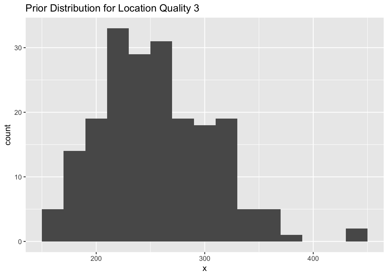
Figure 2.3: A histogram representing a prior distribution (normal) for location quality class 3 with a mean of log(250) and standard error of 0.2.
qual_2 <- data.frame( x = exp(rnorm(200,log(1500),0.2)))
ggplot(data = qual_2, aes(x=x)) + geom_histogram(binwidth = 20) +
  ggtitle("Prior Distribution for Location Quality 1")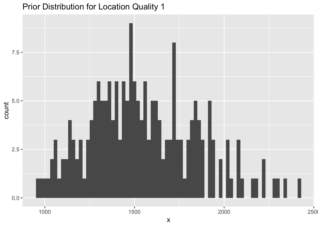
Figure 2.4: (ref:histogram-qual-1-prior)
qual_B <- data.frame( x = exp(rnorm(200,log(2500),0.4)))
ggplot(data = qual_B, aes(x=x)) + geom_histogram(binwidth = 20) +
  ggtitle("Prior Distribution for Location Quality B")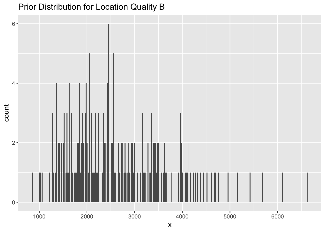
Figure 2.5: A histogram representing a prior distribution (normal) for location quality class B with a mean of log(2500) and standard error of 0.4.
In addition to prior distributions for the location quality classes, we can also provide a prior distribution for the beta parameter. We suggest a normal distribution with a mean of -4 and a standard deviation of 2. This encourages the model to fit a smoother track unless the data warrant a rougher, more Brownian, path.
beta <- data.frame( x = exp(rnorm(200,-4,2)))
ggplot(data = beta, aes(x=x)) + geom_histogram(binwidth = 20) +
  ggtitle("Prior Distribution for Beta Parameter")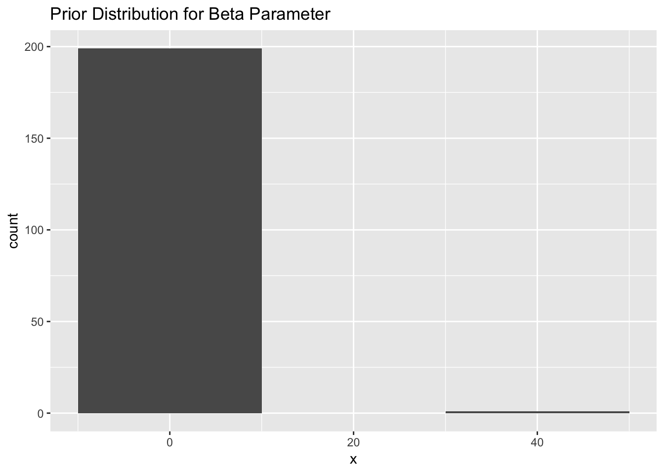
Figure 2.6: A histogram representing a prior distribution (normal) for the beta parameter with a mean of -4 and standard error of 2.
2.5.4.2 Prior Distributions vs Fixed Values and Constraints
Previous documentation and examples that described a setup for ‘crawl’ often suggested users implement a mixed approach by providing both fixed values and constraints to optimize the fit and increase the model’s ability to converge with limited/challenging data. We now suggest users rely on prior distributions to achieve a similar intent but provide the model more flexibility. Users should feel free to explore various distributions and approaches for describing the priors (e.g. laplace, log-normal) based on their data and research questions.
Those documents also often suggested fixing the beta parameter to 4 as the best approach to encourage challenging datasets to fit. This, essentially, forced the fit toward Brownian movement. We now suggest users rely on the prior distribution centered on -4 (smoother fit) and, if needed, fix the beta parameter to -4. Only fix the parameter to 4 as a final resort.
2.6 Fitting with crawl::crwMLE()
The crawl::crwMLE() function is the workhorse for fitting our observed data to
a continuous-time correlated random walk model. At this point, we have our data
structure setup and we’ve established our initial parameters, specified fixed
values for any parameters we will not estimate, and provided some constraints
on those parameter estimates.
Instead of calling crawl::crwMLE() directly, we will create a wrapper function
that will work better with our tidy approach. It also allows us to make
sequencial calls to crawl::crwMLE() that adjust parameters in cases where the
fit fails.
A few other aspects about our wrapper function to note. We pass our observed
data in as d and then the parameters fixpar, and constr.
Additionally, we can specify tryBrownian = FALSE if we don’t want the model
to fit with Brownian motion as the final try.
Each of the prior functions is specified within the function and the function
cycles through a for loop of calls to crawl::crwMLE() with each prior. Note,
the first prior value is NULL to specify our first model fit try is without
any prior.
Our wrapper function also checks the observed data, d, for any activity
column to determine whether activity parameter should be included in the
model fit.
fit_crawl <- function(d, fixpar) {

## if relying on a prior for location quality
## replace this with the function described previously
prior <- function(p) {
  dnorm(p[2], -4, 2, log = TRUE)
}

fit <- crawl::crwMLE(
  mov.model =  ~ 1,
  err.model = list(
      x =  ~ ln.sd.x - 1,
      y =  ~ ln.sd.y - 1,
      rho =  ~ error.corr
    ),
  if (any(colnames(d) == "activity")) {
        activity <- ~ I(activity)
      } else {activity <- NULL},
  fixPar = fixpar,
  data = d,
  method = "Nelder-Mead",
  Time.name = "date_time",
  prior = prior,
  attempts = 8,
  control = list(
    trace = 0
  ),
  initialSANN = list(
    maxit = 1500,
    trace = 0
  )
)
fit
}
The tidy and purrrific approach to model fitting is to store the model results and estimated parameters as a list-column within our nested tibble. This has the significant benefit of keeping all our data, model specifications, model fits, parameter estimates — and, next, our model predictions — nicely organized.
library(pander)
tbl_locs_fit <- sf_locs %>%
  dplyr::mutate(fit = furrr::future_pmap(list(d = data,fixpar = fixpar),
                           fit_crawl),
                params = map(fit, crawl::tidy_crwFit))
After successfully fitting our models, we can explore the parameter estimates that are a result of that fit. The first set of tables are for our two seal deployments and the model has been fit without any activity data.
panderOptions('knitr.auto.asis', FALSE)
tbl_locs_fit$params %>%
walk(pander::pander,caption = "crwMLE fit parameters")| term | estimate | std.error | conf.low | conf.high |
|---|---|---|---|---|
| ln tau.x ln.sd.x | 1 | NA | NA | NA |
| ln tau.y ln.sd.y | 1 | NA | NA | NA |
| ln sigma (Intercept) | 7.279 | 0.014 | 7.252 | 7.306 |
| ln beta (Intercept) | 4.277 | 0.591 | 3.118 | 5.436 |
| logLik | -46741 | NA | NA | NA |
| AIC | 93487 | NA | NA | NA |
| term | estimate | std.error | conf.low | conf.high |
|---|---|---|---|---|
| ln tau.x ln.sd.x | 1 | NA | NA | NA |
| ln tau.y ln.sd.y | 1 | NA | NA | NA |
| ln sigma (Intercept) | 7.611 | 0.045 | 7.522 | 7.7 |
| ln beta (Intercept) | -0.74 | 0.115 | -0.967 | -0.514 |
| logLik | -15491 | NA | NA | NA |
| AIC | 30986 | NA | NA | NA |
Our second set of tables are for our two seal deployments and the model has been fit with inclusion of activity data.
tbl_locs_activity_fit <- tbl_locs_activity %>%
  dplyr::mutate(fit = furrr::future_pmap(list(d = data,fixpar = fixpar),
                           fit_crawl),
params = map(fit, crawl::tidy_crwFit))panderOptions('knitr.auto.asis', FALSE)
tbl_locs_activity_fit$params %>%
walk(pander::pander,caption = "crwMLE fit parameters")| term | estimate | std.error | conf.low | conf.high |
|---|---|---|---|---|
| ln tau.x ln.sd.x | 1 | NA | NA | NA |
| ln tau.y ln.sd.y | 1 | NA | NA | NA |
| ln sigma (Intercept) | 7.281 | 0.014 | 7.254 | 7.308 |
| ln beta (Intercept) | 4.315 | 0.631 | 3.079 | 5.551 |
| ln phi | 0 | NA | NA | NA |
| logLik | -46622 | NA | NA | NA |
| AIC | 93248 | NA | NA | NA |
| term | estimate | std.error | conf.low | conf.high |
|---|---|---|---|---|
| ln tau.x ln.sd.x | 1 | NA | NA | NA |
| ln tau.y ln.sd.y | 1 | NA | NA | NA |
| ln sigma (Intercept) | 7.623 | 0.046 | 7.533 | 7.712 |
| ln beta (Intercept) | -0.767 | 0.115 | -0.991 | -0.542 |
| ln phi | 0 | NA | NA | NA |
| logLik | -15403 | NA | NA | NA |
| AIC | 30809 | NA | NA | NA |
2.7 Exploring and Troubleshooting Model Results
2.8 Predicting a Movement Track
At this point, we have a fitted model for each seal and the next obvious step
is to visualize and explore the resulting fitted track. To accomplish this,
we’ll rely on the crawl::crwPredict() function. This function requires two
key arguments: an object.crwFit and a predTime argument. The first is
simply the fit object from our model fit. The second can be one of two types:
- a vector of POSIXct or numeric values that provide additional prediction times beyond the times for our observed locations in the original data. This vector should not start before the first observation or end after the last observation.
- if the original data were provided as a POSIXct type (which, in this example,
they were), then
crawl::crwPredict()can derive a sequence of regularly spaced prediction times from the original data. The user only needs to provide a character string that describes the regularly spaced duration. This character string should correspond to thebyargument of theseq.POSIXtfunction (e.g. ‘1 hour’, ‘30 mins’).
tbl_locs_fit <- tbl_locs_fit %>%
  dplyr::mutate(predict = furrr::future_map(fit,
                                     crawl::crwPredict,
                                     predTime = '1 hour'))
We still need to perform some additional processing of the prediction object
before we can use the information in analysis or visualize the track. We will
create a custom function as.sf() which will convert our crwPredict object
into an sf object of either “POINT” or “MULTILINESTRING”
tbl_locs_fit <- tbl_locs_fit %>%
  dplyr::mutate(sf_points = purrr::map(predict,
                                       crawl::crw_as_sf,
                                       ftype = "POINT",
                                       locType = "p"),
                sf_line = purrr::map(predict,
                                     crawl::crw_as_sf,
                                     ftype = "LINESTRING",
                                     locType = "p")
                )
sf_pred_lines <- do.call(rbind,tbl_locs_fit$sf_line) %>%
mutate(id = tbl_locs_fit$deployid) %>%
rename(deployid = id)
sf_pred_points <- tbl_locs_fit %>% tidyr::unnest(sf_points) %>%
mutate(geometry = sf::st_sfc(geometry)) %>%
sf::st_as_sf() %>% sf::st_set_crs(3571)esri_ocean <- paste0('https://services.arcgisonline.com/arcgis/rest/services/',
'Ocean/World_Ocean_Base/MapServer/tile/${z}/${y}/${x}.jpeg')
ggplot() +
annotation_map_tile(type = esri_ocean,zoomin = 1,progress = "none") +
layer_spatial(sf_pred_lines, size = 0.75,aes(color = deployid)) +
scale_x_continuous(expand = expand_scale(mult = c(.6, .6))) +
scale_y_continuous(expand = expand_scale(mult = c(0.35, 0.35))) +
scale_color_brewer(palette = "Dark2") +
theme(legend.position = "none") +
ggtitle("Predicted Location Paths",
subtitle = "harbor seals (n=2), Aleutian Islands, Alaska, USA")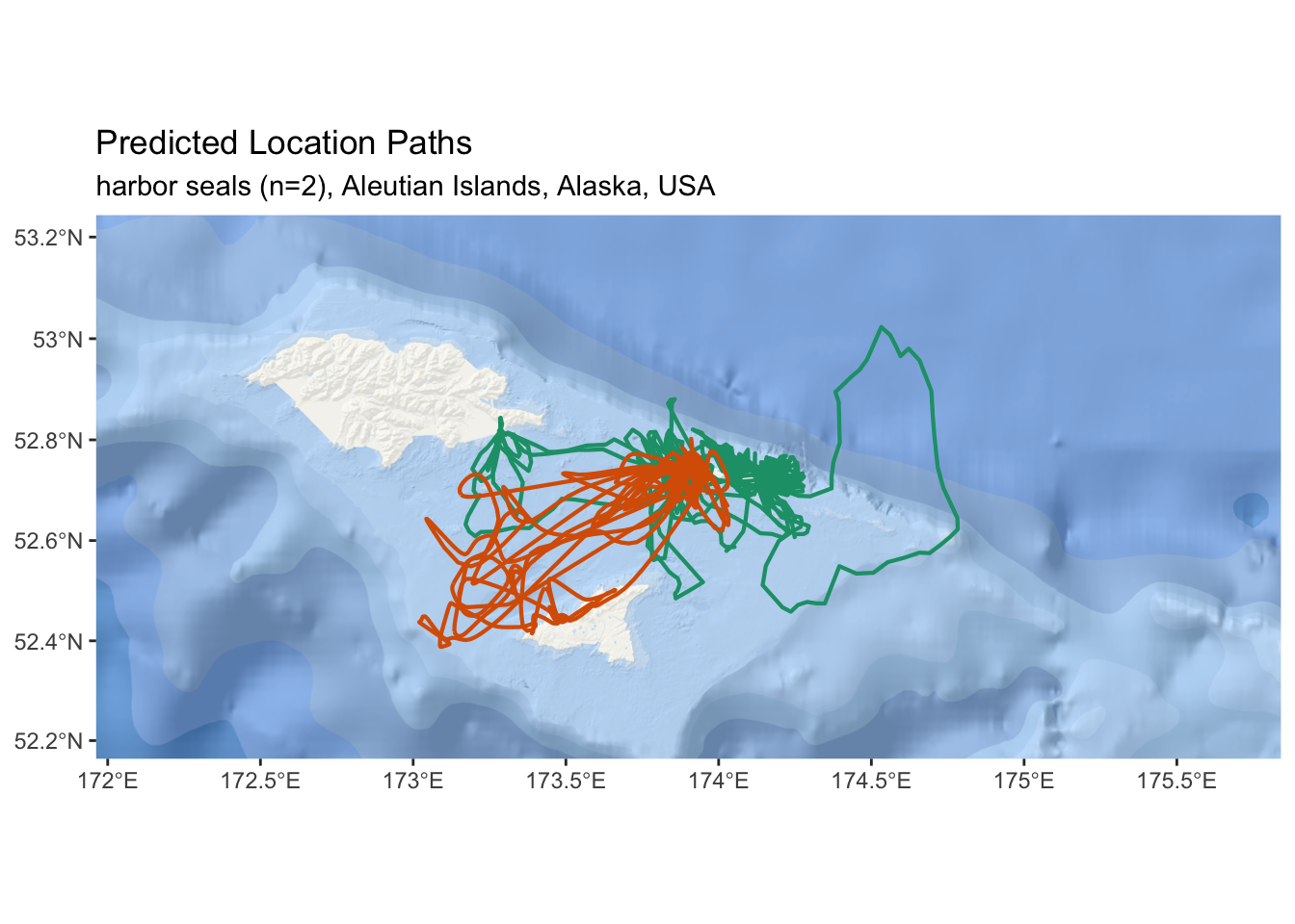
Figure 2.7: An interactive map of predicted tracks from two harbor seals in the Aleutian Islands.
2.9 Simulating Tracks from the Posterior
.get_sim_tracks <- function(crw_fit,iter) {

  simObj <- crw_fit %>% crawl::crwSimulator(predTime = '1 hour')

  sim_tracks = list()
  for (i in 1:iter) {
    sim_tracks[[i]] <- crawl::crwPostIS(simObj, fullPost = FALSE)
  }
  return(sim_tracks)
}

tbl_locs_fit <- tbl_locs_fit %>%
  dplyr::mutate(sim_tracks = purrr::map(fit,
                                       .get_sim_tracks,
                                       iter = 5))

tbl_locs_fit <- tbl_locs_fit %>%
  dplyr::mutate(sim_lines = crawl::crw_as_sf(.$sim_tracks, ftype = "MULTILINESTRING",
                                             locType = "p"))
2.10 Visualization of Results
sf_sim_lines <- do.call(rbind,tbl_locs_fit$sim_lines) %>%
  mutate(id = tbl_locs_fit$deployid) %>%
  rename(deployid = id)

esri_ocean <- paste0('https://services.arcgisonline.com/arcgis/rest/services/',
                     'Ocean/World_Ocean_Base/MapServer/tile/${z}/${y}/${x}.jpeg')

ggplot() +
  annotation_map_tile(type = esri_ocean,zoomin = 1,progress = "none") +
  layer_spatial(sf_sim_lines, size = 0.25, alpha = 0.1, aes(color = deployid)) +
  facet_grid(rows = vars(deployid)) +
  scale_x_continuous(expand = expand_scale(mult = c(.6, .6))) +
  scale_y_continuous(expand = expand_scale(mult = c(0.35, 0.35))) +
  scale_color_brewer(palette = "Dark2") +
  theme(legend.position = "none") +
  ggtitle("Simulated Location Paths",
          subtitle = "harbor seals (n=2), Aleutian Islands, Alaska, USA")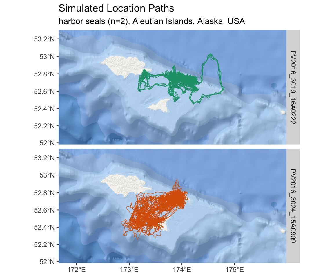
Figure 2.8: An interactive map of simulated tracks from two harbor seals in the Aleutian Islands.