Re-routing Harbor Seal Movement Tracks Around Land with {pathroutr}

Alaska Harbor Seal Example

Essential Packages

This example relies on a non-release version of {crawl}

# not run
library(remotes)
install_github('NMML/crawl@devel')

library(crawl)
library(sfnetworks)
library(pathroutr)

Additional packages we’ll want to load

library(dplyr)
library(sf)
library(ggplot2)
library(ggspatial)
library(dplyr)

The purpose of this is to demonstrate a more ‘real world’ use of {pathroutr} for re-routing of marine animal movement around land features. Here, we will use the Alaska harbor seal data provided in the {crawl} package to:

1. demonstrate the data wrangling and pre-processing needed
2. use {crawl}’s movement model to predict the most likely path
3. re-route the predicted path around any land barriers
4. repeat the process but using {crawl}’s multiple imputation functionality to create a set of possible predicted paths that span model uncertainty

Pre-processing Track Data and Land Polygon Data

For our land data, we will source in the Alaska 1:250000 coastal data polygon. This is provided by the Alaska Department of Natural Resources and was obtained from their open data portal (https://gis.data.alaska.gov/datasets/alaska-1250000). The commented code provides a query to pull the data directly from the portal API. Note, only those polygons that intersect with the bounding box of our harbor seal movement are included.

NOTE: because this step is time consuming, we will load directly from package data

# akcoast_qry <- "https://arcgis.dnr.alaska.gov/arcgis/rest/services/OpenData/Physical_AlaskaCoast/MapServer/2/query?where=1%3D1&outFields=*&geometry=-159.240%2C55.112%2C-152.422%2C59.413&geometryType=esriGeometryEnvelope&inSR=4326&spatialRel=esriSpatialRelIntersects&outSR=3338&f=json"
# 
# akcoast <- sf::read_sf(akcoast_qry)
# akcoast <- sf::st_make_valid(akcoast)
data("akcoast")

Now, let’s load in our harbor seal data from the {crawl} package. The harborSeal_sf data is only available in the devel branch. We also transform to EPSG:3338.

data("harborSeal_sf")

harborSeal_sf <- harborSeal_sf %>% sf::st_transform(3338)

Let’s plot things to make sure everything looks good. The harborSeal_sf data has missing values in the geometry field so we need to filter those out when making a line.

l <- harborSeal_sf %>% 
  dplyr::filter(!sf::st_is_empty(.)) %>% 
  dplyr::summarise(do_union = FALSE) %>% 
  sf::st_cast('LINESTRING')

ggplot() +
  ggspatial::annotation_spatial(akcoast, fill = "cornsilk3", size = 0) +
  ggspatial::layer_spatial(l, color = "darkgrey", size = 0.5) +
  ggspatial::layer_spatial(harborSeal_sf, color = "deepskyblue3", size = 0.5) +
  theme_void()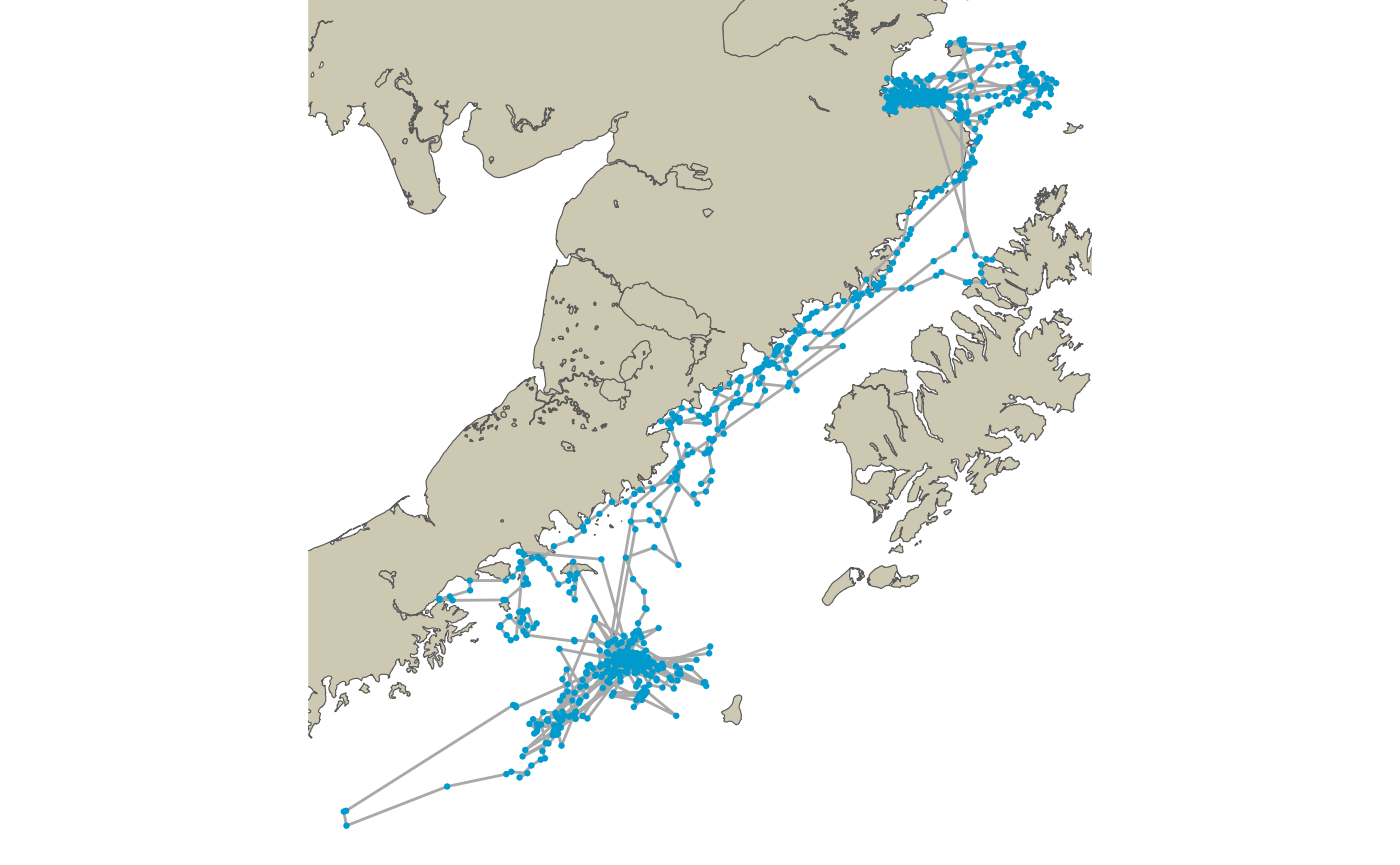

Movement data from a harbor seal in Alaska. Raw Argos observations and the derived connect-the-dots trackline

Re-Route Raw Argos Observations

While the preferred approach would be to rely on a movement model for predicting the path of our seal, it can sometimes be useful to just correct the raw observations. So, that’s what we’ll do first.

Limit Barrier Polygon to Region of Interest

With such a large geographic area, the computational time needed to create our visibility graph could be quite large. So, we will want to limit our land polygon as much as we reasonably can.

We’ll do this by creating a convex hull boundary around our observed data and limiting the region to this space. Here, we’ll go with a buffer of 50 km around each point and rely on the buffered features to create our convex hull. The size of the buffer is case-specific. In this case, we could likely get away with a smaller buffer if we were only interested in the connect-the-dot track or a model predication. But, later, we will also impute additional, possible tracks from the model fit to better represent model uncertainty. For this reason, we went with a larger buffer so we only have to create a single network graph.

land_region <- sf::st_buffer(harborSeal_sf, dist = 50000) %>% 
  sf::st_union() %>% 
  sf::st_convex_hull() %>% 
  sf::st_intersection(akcoast) %>% 
  st_collection_extract('POLYGON') %>% 
  st_sf()

ggplot() +
  ggspatial::annotation_spatial(land_region, fill = "cornsilk3", size = 0) +
  ggspatial::layer_spatial(l, color = "darkgrey", size = 0.5) +
  ggspatial::layer_spatial(harborSeal_sf, color = "deepskyblue3", size = 0.5) +
  theme_void()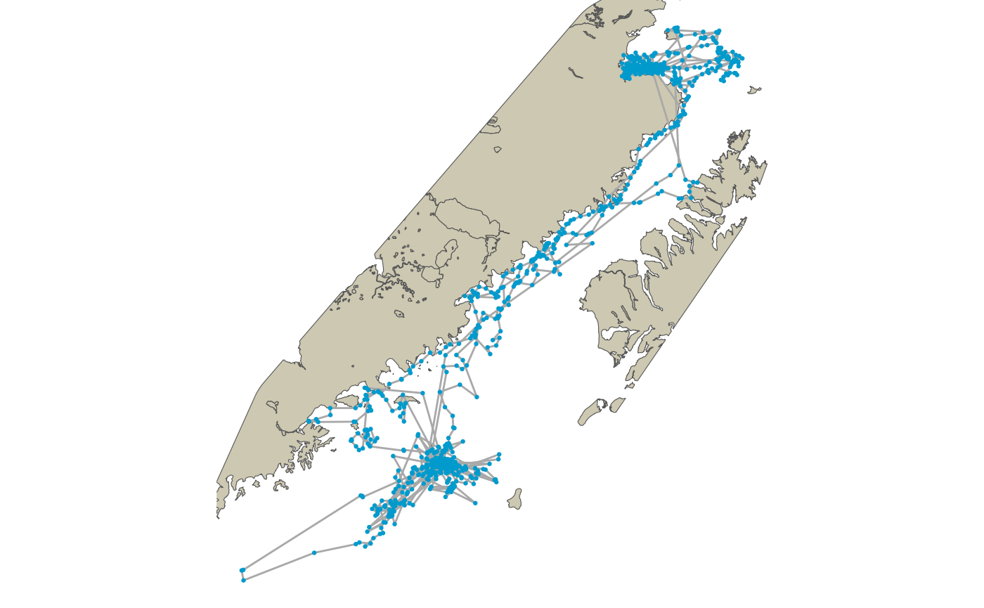

Land barrier polygon after limiting to a 50km buffered convex hull of the observation points

Create Visibility Graph

At this point, we are ready to create our visibility graph using the pathroutr::prt_visgraph() function. We’ll keep centroids = FALSE in order to speed up the build. Adding additional centroids will increase the likelihood of linearity in the calculated shortest path. This is especially true when the shortest path crosses larger areas of open water. However, adding the additional centroids results in a very large increase in computational time (both in creation of the visual graph and in subsequent operations). There is likely little improvement in situations where the shortest path routing follows the coast. The default setting is centroids=FALSE. If a user chooses to set centroids=TRUE, we strongly encourage setting centroid_limit to a large value (default is 1e+07).

vis_graph <- prt_visgraph(land_region)

Let’s take a look at our network. The network stores both “nodes” and “edges” and we need to “activate” one or the other before converting to a simple feature collection.

vis_graph_sf <- sfnetworks::activate(vis_graph,"edges") %>% sf::st_as_sf()

ggplot() +
  ggspatial::annotation_spatial(land_region, fill = "cornsilk3", size = 0) +
  ggspatial::layer_spatial(vis_graph_sf, size = 0.5) +
  theme_void()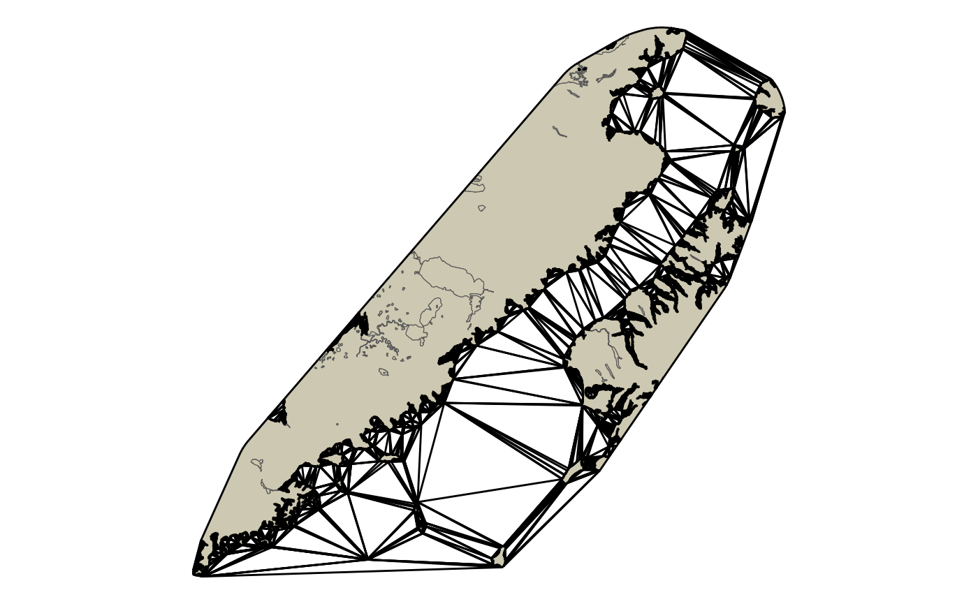

Visibility graph network edges created with the sfnetworks package. All vertices from the land polygon were used as nodes in the network and any edges that crossed land were removed.

Note the large triangles in the large, open water areas. This is a key advantage for our purpose as we concentrate the detail of our network along the coastline where routing of our tracks around land requires the most detail. The trade-off is that any shortest path routing that crosses the large, open areas will have less linearity. If we had set centroids=TRUE, then a centroid point would have been added to each of these triangles and the mesh would have been rebuilt to include those points.

Determine Segments of Track On Land

In this example, our interest is to re-route only the portions of the track that cross land. So, we need to identify the segments of consecutive points on land and, also, the points in water that bookend each segment. We will use this information to calculate our shortest path through our network and create an updated series of point features.

track_pts <- harborSeal_sf %>% dplyr::filter(!sf::st_is_empty(.))
segs_tbl <- get_barrier_segments(track_pts,land_region)
segs_tbl
#> # A tibble: 44 × 6
#>      sid start_idx end_idx n_pts             start_pt
#>    <int>     <dbl>   <dbl> <dbl>          <POINT [m]>
#>  1     1        70      72     1  (-7141.435 1009874)
#>  2     2       211     213     1   (17825.82 1009686)
#>  3     3       296     298     1 (-166514.5 678462.8)
#>  4     4       299     301     1 (-166385.8 678569.6)
#>  5     5       310     312     1   (-159772 672617.8)
#>  6     6       313     315     1 (-168417.8 679098.1)
#>  7     7       346     348     1 (-166934.5 680376.9)
#>  8     8       372     375     2   (-167836 679632.4)
#>  9     9       390     392     1   (-164953 673937.4)
#> 10    10       398     400     1   (-163341.9 680010)
#> # ℹ 34 more rows
#> # ℹ 1 more variable: end_pt <POINT [m]>

Determine Re-routed Track via Shortest Path

Since our bookend points were not used to create our visibility graph, we need to also determine the closest network node to each point. Our prt_nearestnode() function relies on the nabor::knn() function for this. The user does not need to call this explicitly as it is handled within the prt_shortpath() function.

Now, we have all the information we need to calculate the shortest path through our network for each segment. The igraph::shortest_paths() function calculates and returns the series of edges that make up the shortest path (by distance) from the start node to the end node. The prt_shortpath() function wraps in additional functionality (e.g. blending the network, identifying the nearest nodes to our start and end points, assembling the path, extending the path at each end to connect with our bookend points).

segs_tbl <- segs_tbl %>% prt_shortpath(vis_graph)

ggplot() + 
  ggspatial::annotation_spatial(land_region, fill = "cornsilk3", size = 0) +
  ggspatial::layer_spatial(segs_tbl$geometry, color = "deepskyblue3") +
  theme_void()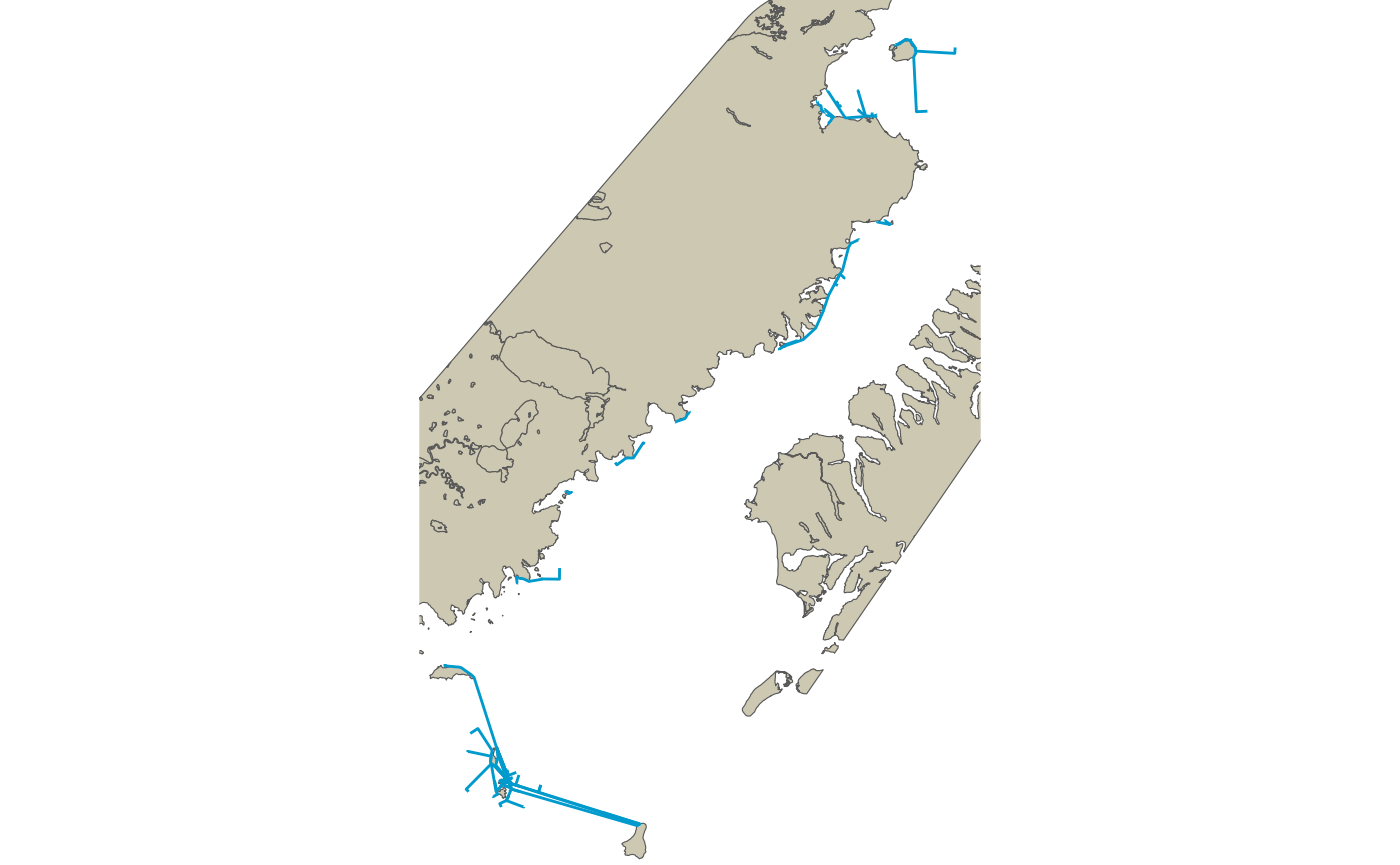

Segments that were identified to cross land have been re-routed along the shortest path throught visibility network

Update Geometry With Re-routed Coordinates

In reality, most of the time the user will simply want to provide an ordered series of points, a barrier polygon, and the spatial network. {pathroutr} includes a convenience function for this, prt_reroute(). This will return a two-column tibble with an index location and geometry for each re-routed point. The user can use this to update the original data as they see fit. Or, the prt_update_points() function can be used to replace the geometry in place. This last step is done by inserting the fixed points back into our original path. We take the number of points in the original segment and distribute an equal number of points along the updated path. Because the geometry in the original dataset is updated in place, some users may want to create customized functions or workflows to better track updates to the original data.

track_pts_fix <- prt_reroute(track_pts, land_region, vis_graph)

track_pts_fix <- prt_update_points(track_pts_fix, track_pts)

track_line_fixed <- track_pts_fix %>% summarise(do_union = FALSE) %>% st_cast('LINESTRING')

ggplot() +
  ggspatial::annotation_spatial(land_region, fill = "cornsilk3", size = 0) +
  ggspatial::layer_spatial(track_line_fixed, color = "darkgrey", size = 0.5) +
  ggspatial::layer_spatial(track_pts_fix, color = "deepskyblue3", size = 0.5) +
  theme_void()

Raw Argos observation geometries updated in place with the re-routed paths

Re-Routing a Movement Model Prediction

Now, we’ll move on to the preferred workflow and establish a movement model from our raw location observations.

Here, we rely on an example from the {crawl} package. But, other model approaches (e.g. {foieGras}) should work as well. We have plans to provide specific methods for a variety of model outputs in future releases.

Fit Movement Model and Predict Locations

As you might have noticed when we re-routed our raw observations, the trackline derived from those points can still cross land. This is because we only control for the presence of observation points on land. At the irregular and sometimes large time intervals common to location data for marine mammals, this cannot be avoided. However, once we have a movement model, we can predicted a finer location intervals and limit this possibility. You will notice in this example, the prediction interval is every 15 minutes.

##Fit model as given in Johnson et al. (2008) Ecology 89:1208-1215
## Start values for theta come from the estimates in Johnson et al. (2008)
fixPar = c(log(250), log(500), log(1500), rep(NA,5), 0)
displayPar( mov.model=~1, err.model=list(x=~Argos_loc_class-1),data=harborSeal_sf, 
            activity=~I(1-DryTime),fixPar=fixPar)
#>                  ParNames   fixPar thetaIdx
#> 1 ln tau Argos_loc_class0 5.521461       NA
#> 2 ln tau Argos_loc_class1 6.214608       NA
#> 3 ln tau Argos_loc_class2 7.313220       NA
#> 4 ln tau Argos_loc_class3       NA        1
#> 5 ln tau Argos_loc_classA       NA        2
#> 6 ln tau Argos_loc_classB       NA        3
#> 7    ln sigma (Intercept)       NA        4
#> 8     ln beta (Intercept)       NA        5
#> 9                  ln phi 0.000000       NA
constr=list(
  lower=c(rep(log(1500),3), rep(-Inf,2)),
  upper=rep(Inf,5)
)

set.seed(123)
fit1 <- crwMLE(
  mov.model=~1, err.model=list(x=~Argos_loc_class-1), activity=~I(1-DryTime),
  data=harborSeal_sf,  Time.name="Time", 
  fixPar=fixPar, theta=c(rep(log(5000),3),log(3*3600), 0),
  constr=constr, method="L-BFGS-B",
  control=list(maxit=2000, trace=1, REPORT=1)
)
#> Beginning SANN initialization ...
#> Beginning likelihood optimization ...
#> iter    1 value 41202.609844
#> iter    2 value 41056.998394
#> iter    3 value 40756.499672
#> iter    4 value 40146.411888
#> iter    5 value 40066.268387
#> iter    6 value 40005.050127
#> iter    7 value 40001.092459
#> iter    8 value 40001.050325
#> iter    9 value 40001.048541
#> iter   10 value 40001.048534
#> final  value 40001.048534 
#> converged

pred1 = crwPredict(fit1, predTime = '15 min')
pred1_sf <- pred1 %>% crw_as_sf("POINT","p")

Identify Predicted Locations on Land

As before, we need to identify all of the segments of consecutive locations on land and determine the associated start and end nodes within our network.

segs_tbl <- get_barrier_segments(pred1_sf,land_region)
segs_tbl
#> # A tibble: 140 × 6
#>      sid start_idx end_idx n_pts             start_pt
#>    <int>     <dbl>   <dbl> <dbl>          <POINT [m]>
#>  1     1      2426    2435     8   (16195.24 1008923)
#>  2     2      2482    2485     2   (13845.85 1009221)
#>  3     3      2486    2488     1   (14334.24 1007460)
#>  4     4      2488    2557    68   (14625.18 1006411)
#>  5     5      2648    2651     2    (47203.07 912631)
#>  6     6      2656    2662     5  (44653.54 904336.9)
#>  7     7      3260    3263     2 (-169713.6 678313.5)
#>  8     8      3524    3531     6   (-166814 672859.7)
#>  9     9      3545    3564    18 (-166337.5 678529.5)
#> 10    10      3610    3616     5 (-166162.5 678383.6)
#> # ℹ 130 more rows
#> # ℹ 1 more variable: end_pt <POINT [m]>

Re-route Model Prediction via Shortest Path

And just like we did with the raw observations, we use the prt_shortpath() function to calculate all of our re-routed paths

segs_tbl <- segs_tbl %>% prt_shortpath(vis_graph)

ggplot() + 
  ggspatial::annotation_spatial(land_region, fill = "cornsilk3", size = 0) +
  ggspatial::layer_spatial(segs_tbl$geometry, color = "deepskyblue3") +
  theme_void()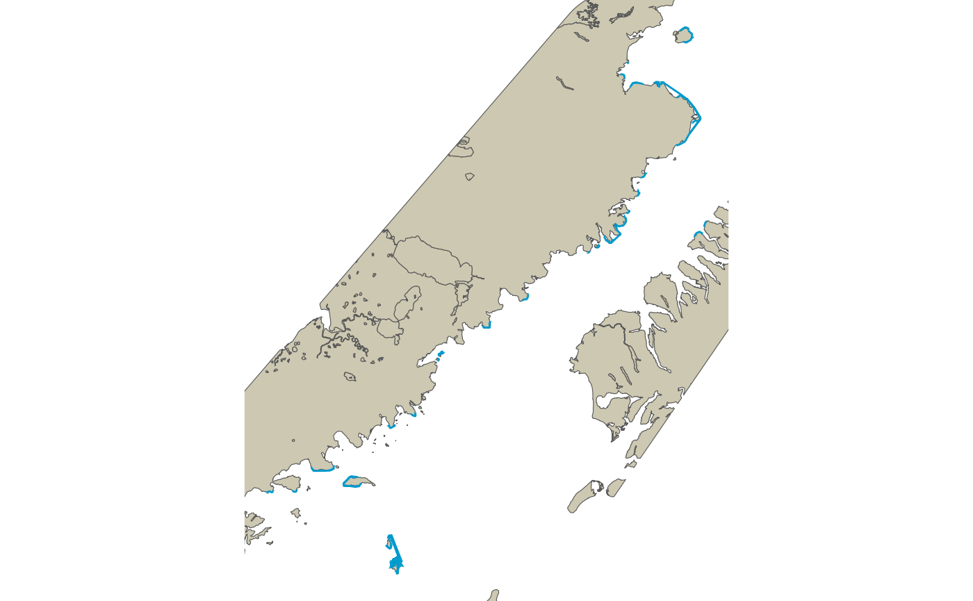

Re-routed segments from the predicted path

Update Predicted Path

As in the first example, we could have skipped these last few steps and just relied on the prt_reroute() and prt_update_points() functions.

track_pts_fix <- prt_reroute(pred1_sf, land_region, vis_graph)

track_pts_fix <- prt_update_points(track_pts_fix, pred1_sf)

track_line_fixed <- track_pts_fix %>% summarise(do_union = FALSE) %>% st_cast('LINESTRING')

ggplot() +
  ggspatial::annotation_spatial(land_region, fill = "cornsilk3", size = 0) +
  ggspatial::layer_spatial(track_line_fixed, color = "deepskyblue3", size = 0.5) + 
  theme_void()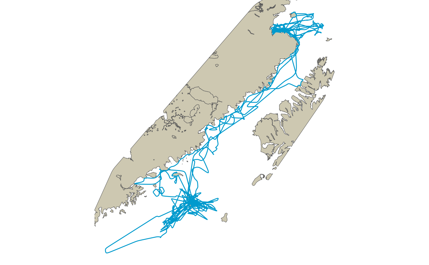

Updated predicted path with re-routed geometries

Multiple Imputation

The recommended analytic workflow for {crawl} movement models is to characterize movement from a collection of imputed paths from the model fit. The {pathroutr} re-routing can be applied to each of these imputed paths and, hopefully, provide a more complete picture of uncertainty.

Create Multiple Imputations from {crawl} Model

We will use the crawl::crwSimulator() and crawl::crwPostIS() functions to create our imputed paths. The code below is a more tidyverse-centric approach that relies on dplyr::rowwise() and dplyr::mutate() to draw and, then, re-route 5 imputed paths. Note, here, we set blend = FALSE for the prt_reroute() function call. This is just to save some computation time for this example.

crw_sim <- crawl::crwSimulator(fit1, predTime = "15 min")
#> Computing importance weights ...

imputes <- tibble::tibble(.rows = 5) %>% 
  dplyr::rowwise() %>% 
  mutate(postis = list(crwPostIS(crw_sim, fullPost = FALSE)),
         pts = list(crw_as_sf(postis, locType = "p", ftype = "POINT")),
         rrt_pts = list(prt_reroute(pts, land_region, vis_graph, blend = FALSE)),
         pts_fix = list(prt_update_points(rrt_pts, pts)),
         lines_fix = list(pts_fix %>% summarise(do_union = FALSE) %>% st_cast('LINESTRING'))
         )

sim_lines <- do.call(rbind, imputes$lines_fix)

The figure below combines our predicted path and the collection of five imputed paths. Note the routing of tracks around the land barrier features for both the predicted track and the imputed tracks. One thing to keep in mind is that the imputed tracks will often have less linear inertia and, thus, a greater number of small land crossings. This means re-routing any one of the imputed tracks will likely take longer than the predicted path. The exact number of imputed paths needed will be case specific. However, more than 20 is likely not needed.

ggplot() +
  ggspatial::annotation_spatial(land_region, fill = "cornsilk3", size = 0) +
  ggspatial::layer_spatial(sim_lines, color = "deepskyblue", alpha = 0.35) +
  ggspatial::layer_spatial(track_line_fixed, color = "deepskyblue3", size = 0.5) + 
  theme_void()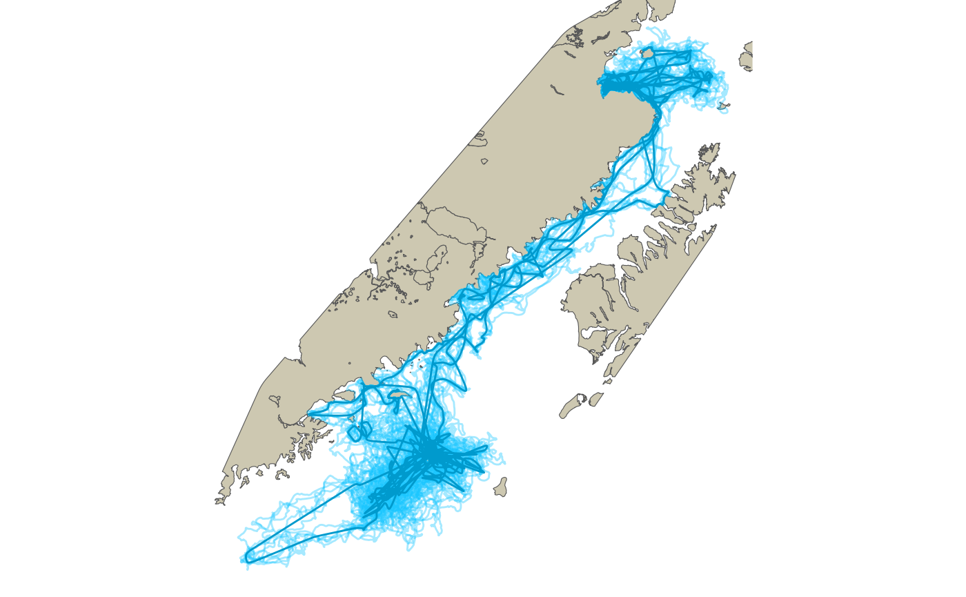

Five imputed paths are shown along with the predicted most likely path after re-routing around the land barrier.

Space Use Analysis

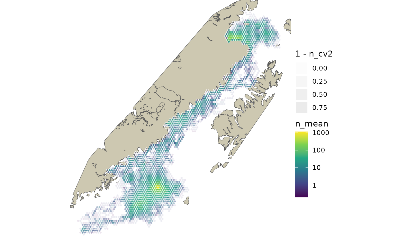
Understanding space use is a common goal for telemetry data like is presented in this example. Since the movement model allows us to predict at regular intervals, we can use the count of predicted points within a regular grid to represent space use. And, by averaging the count across multiple imputed paths we can create a space use surface that incorporates our uncertainty.

First thing we’ll want to do is to create a regular grid for our the bounding box of our study area. It is important to base this grid on sim_lines so that we have complete spatial coverage for our imputed tracks. We’ll use a hexagonal grid and remove all of the grid cells that fall within our land polygon. This will leave those cells that are completely over water or that touch or overlap the coastline.

hex_grid <- sf::st_make_grid(
  st_as_sfc(st_bbox(sim_lines)),
  cellsize = 5000,
  square = FALSE
) %>% st_sf() %>% 
  st_filter(st_union(land_region), .predicate = pathroutr:::not_within) %>% 
  tibble::rowid_to_column(var = "hexid")

Now, we need to join our fixed points from our imputations (imputes$pts_fix) to our hex_grid and count the number of points per grid cell.

# Suppress summarise info
options(dplyr.summarise.inform = FALSE)

hexbins <- imputes$pts_fix %>% purrr::map(~ {
  st_join(.x, hex_grid, join = st_intersects) %>% 
    sf::st_set_geometry(NULL) %>% 
    group_by(hexid) %>% 
    summarise(n = n()) %>% 
    right_join(hex_grid, by = "hexid") %>% 
    sf::st_sf()})

For our seal-use statistics, we’ll want to average our counts per grid cell across each of the imputed tracks. We will also calculate standard deviation, CV, and a normalized CV that we will use in our plot to communicate uncertainty.

seal_use <- do.call(rbind, hexbins) %>% 
  mutate(n = ifelse(is.na(n),0,n)) %>% 
  group_by(hexid) %>% summarise(n_mean = mean(n), n_sd = sd(n)) %>% 
  dplyr::filter(n_mean > 0) %>% 
  dplyr::mutate(n_cv = n_sd/n_mean,
                n_cv2 = n_cv/max(n_cv))

Our final plot of seal use is presented on a log10 scale and the transparency is set based on our normalized CV such that cells with higher uncertainty are more transparent.

ggplot() +
  ggspatial::annotation_spatial(land_region, fill = "cornsilk3", size = 0) +
  ggspatial::layer_spatial(seal_use, 
                           aes(fill = n_mean, alpha = 1 - n_cv2), color = "white", size = 0.05) + 
  scale_fill_viridis_c(trans = "log10") +
  theme_void()